Activity 6 - Properties and Applications of the 2D Fourier Transform

Hi there visitor! This activity is just a continuation and somehow a more advanced version of Activity 5 wherein we tend to explore more on the deeper properties and characteristics of the Fourier Transform.

First of all I would not start my blog with a certain life lesson or realization due time limitations. Well, I guess the main point here is that sometimes, no matter how Fast we think we are in Transforming, we must realize that there will be certain moments that we need to accept our limitations and do our best in the midst of the unwanted circumstances.


ANAMORPHIC PROPERTY OF THE FOURIER TRANSFORM

The Anamorphic properties of the FT just tells us the inverse properties of the FT wherein if a certain dimension longer at the digital space, it will tend to be shorter in the Fourier space, and vice versa. We can see this in Figure 1 below wherein the corresponding patterns on the left, with their FT on the right.

Figure 1. (Top to bottom) Tall and wide rectangles, and two dots symmetrically separated from the center, with their corresponding Fourier transforms. 

The theoretical expectation is met upon examining the shift in the dominant, longer dimension in the Fourier space which can be obviously implied in the long and wide rectangles. The two dots tend to have an FT that is a sinusoidal pattern along the x-axis. Anamorphism can be seen upon observing Figure 2 that shows a decrease in the line widths of the FT (bottom) upon increasing the gap between the two dots (top).

Figure 2. Two dots (top) and its corresponding FT (bottom) showing a decrease in the line widths in Fourier space upon increasing the dot separation in digital space.

Here's a cool GIF for further visualization of Anamorphism (please take note Aliasing due to very high frequencies of the sinusoid):

ROTATION PROPERTY

Here we explore the rotation property of the FT upon the introduction of rotation parameters and sinusoid addition and overlap. The summary of this part can be observed in Figure 3 which shows (from left to right) the FT of a sinusoid showing peak frequencies (one negative-y and one positive-y: the reason why there are 2 dots), the resulting FT upon adding a constant bias, the FT upon the introduction of a rotational parameter, the FT of combined sinusoids, and the FT of  rotated and combined sinusoids.

Figure 3. The sinusoidal patters(top) and their corresponding FTs (bottom).

Shown below are GIFs for better visualization. 

Sinusoid of increasing frequency with its corresponding FT

Sinusoid with increasing constant bias with its corresponding FT

Sinusoid rotated clockwise with its corresponding FT

Combined sinusoids with one in the x and the other in the y direction with its corresponding FT

Combined and rotated sinusoid with rotational functions and their corresponding FT

Combined and rotated sinusoid with more complicated rotational functions and their corresponding FT

CONVOLUTION THEOREM

Here we revisit and go deeper in the convolution theorem of Fourier Transforms. Figure 4 shows the summary of what we did in this part. (From top to bottom) First, the FT of two Dirac deltas (peak ponts) were obtained then the said points were replaced by first a circle, a square and a gaussian bell curve. The sizes of these patterns were studies and the results were found to still exhibit anamorphism and for very small sizes, they tend to represent almost the FT of the Dirac Delta.

Add caption

LINE REMOVAL THROUGH FOURIER SPACE MASKING

Activity 5 - Fourier Transform Model of Image Formation

They say that the only constant thing in the universe is change. Whoever we are, wherever we're in, or whatever we do, we are always prone to change. From the smallest variations at the subatomic level, to the basic life processes that we do and experience, we always experience change. It seems like whatever we do, we undergo a certain transformation that only varies upon your reference point or to put it simply, your perspective.

Some may look at change in a negative sense, while others might look at it as a positive thing. Our varying perspectives allow us to have the full grasp of the whole image. Personally, I believe that change is good as long as you at least try to understand how it happened. Change will forever be a blur unless you try to experience and engage in it, so that your "transform" will add to your "formation."

Here, we try to transform an image in a literal sense, and upon doing so, we observe and understand multiple properties that are present in the image. We use one of the most popular and easy-to-use models, the Fast Fourier Transform Model in Image Formation.

THE FOURIER TRANSFORM MODEL

On of the most known classes of transform models is the Fourier Transform. It a linear transform that recasts information into another set of linear basis functions. The function of the Fourier Transform (FT) is to convert a physical dimension into the inverse of that dimension. Upon obtaining the FT of a spatial signal, we expect the output to be the inverse space of that signal or particularly its spatial frequency.

In this activity, the FT will be explored with the use of a 2D image.  The FT of an image f(x,y) is given by

where fx and fy  are the spatial frequencies along x and y, respectively. Here, we apply the 2D FT for discrete signals; thus we introduce the discrete FT given by

where k and l are the spatial coordinates along x and y, respectively. Here, M and N are the range of values along, x and y.

Due to the specifications and complexity of the FT model, a certain algorithm, called the Fast Fourier Transform (FFT) algorithm was introduced by Cooley and Turkey for faster FT implementation. The results of this activity essentially show the various characteristics and applications of the FT model with the use of Scilab.

RESULTS

A. FFT Exploration

Figure 1. Compiled results in exploring the properties of FFT for different images.

In this part, I decided to somehow lighten up the mood and be less formal with my writing. Haha. I think that this method would be more efficient in relying my thoughts, especially that this activity is quite a load.

So let's start with figure 1. As you can see, I compiled the images to show the various processes in the part wherein I started to get comfortable with the use of FFT in Scilab. The photos were joined using the old photo joiner (http://old.photojoiner.net/) and Kingsoft Presentation was used to add the labels.

Upon observing the images, it can be seen that the real part of the FFT image greatly resembles the forward FFT image. This is expected because the abs() function was introduced to get the modulus of the complex number, that is of the returned FFT; and the modulus of a complex number is highly influenced by its real part as compared to the imaginary part.  This also tells us that the idea of the whole image of things is not just made up of what we obtain from our senses, what we can observe, or on our own idea of reality, we still need a bit of imagination for us to have the whole grasp of the bigger picture.

REALIZATION!!!

The FFTshift() was also important in obtaining the forward FFT. Initially, without the fftshift() command, I thought that what I was doing was wrong but in reality, I just needed to add a simple command to get the right answer. Huhu. Another realization is boiling…

I guess in life, we focus too much on the complex details and upon experiencing failure, we overthink and overlook the simple solution. Sometimes the best solutions are the simplest ones. 

Yay for simplicity!

Lastly, looking at the rightmost images of the figure, we can see that it's just a vertically inverted image of the original one. This reminds us that in life, there are two types of individuals: the A's and the Circles. The A's are those individuals that upon exerting much effort, they can allow their lives to turn upside-down. Note that this can be both in a positive or negative way. The Circles are the ones that upon exerting much effort they still end up with what they started.

For me, though this whole thing of A's and Circles is just a hypothesis, the outcome is just secondary to the journey. You might end up where you started, or you experienced a certain inversion in life, what matters most is on what you went through and on the priceless knowledge and experiences that you obtained. These things are not perishable and can be considered as true treasures of life.

For further exploration of things, I varied the size of the original image I got quite cool observations and results. I used (GIFCreator.me) in generating the GIF images.

Figure 2. A GIF of the letter A showing the various differences of the FT image with respect to the original image size.

Figure 3. A GIF of a 2D Gaussian bell curve showing the various differences of the FT image with respect to the original image size.

Figures 2 and 3 show that the image size is inversely proportional to the size of the FT image.

Figure 4. A GIF of a centered-circle showing the various differences of the FT image with respect to the original image size.

Here, you can see that though changing the image size has just similar effects to the one in Fig 2, a highly notable change can be seen in the imaginary part of the complex FT image. It can be seen that as the image decreases in size, the patterns formed by the imaginary part does not only zoom-in but also somehow has a form of rotation that leads to pattern variations. Huhu. Beautiful :3

Figure 5. A GIF of a sinusoid along x showing the various differences of the FT image with respect to the original image sinusoid frequency.

The FT of a sinusoid along x (Fig. 5) is composed of three dots with one bright dot in the center and two dimmer dots that somehow "sandwiches" the bright dot. It can be seen that as the frequency increases, the distance of the outer dots with respect to the inner dot also increases. While for Figure 6, I tried to play with the separation distance of the simulated double slit. It can be seen that upon increasing the distance between the slits, the number of maxima values (bright dots) also increases.

Figure 6. A GIF of the simulated double slit showing the various differences of the FT image with respect to the original inter-slit distance

It is also good to note that the square function image acts like two double slits with one along the x and another along the y. This can be seen in the FT image for small square images, but by increasing the size, the maxima values tend to dim, which results in inobservable FT maxima values. 

Figure 7. A GIF of square function showing the various differences of the FT image with respect to the original image size.

B. Convolution

For the convolution, the image below (Figure 8) just shows the effect of the aperture size of a certain camera to the reconstructed image. This shows that ideally, it's better to have higher aperture sizes for you to have higher image resolution and details. Higher aperture size here implies a higher percentage of the rays gathered from the rays reflected off an object. It is also good to note the Fourier image of a centered-circle in Figure 4. As you can see, as the aperture decreases, the resulting image in Fourier space increases in the number of ripples, which in connection to Fig.8 can be seen in the smallest image (leftmost). This is expected because the convolution of two images should look more like the convolved images.

Figure 8. An image showing the aperture of the lens (top) and the corresponding reconstructed (covoluted) image of VIP (bottom)

The idea here is technically straightforward. If you wanna have a clearer view of things, you might want to look at the world through a lens with a wider aperture. Consequently. if you're view of everything seems blurry and unsure, maybe you're just looking at the world with a smaller lens. We all need to increase our field of vision to live the fullness of life.


C. Template Matching


The concept here is finding the letter in the given text where the template letter "A" matches through the use of the correlation function. In the leftmost 2x2 image of Figure 9, it can be seen that the resulting bright spots in the correlated image corresponds to the location where the letter "A" can be found in the text. Upon further exploration, it can be observed that the position of the image that will be correlated should be centered. The middle and rightmost set of 2x2 images show that the correlated images shift to the direction opposite where the image subject for correlation is shifted.

Figure 9. Matched A template with the given set of texts while varying the positions of the A template.

I also explored on the template sizes and as you can observe in figure 10, the result is not size independent, wherein the image template should also be the same size of figure in the larger image upon the correlation process. 

Walang labis, walang kulang. Sakto lang.

Figure 10. Matched A template with the given set of texts while varying the sizes of the A template.

Also, I just wanted to prove that the correlation function is not exclusive to single letters. I applied the same correlation method to two letters (Figure 11) and for face detection (Figure 12).

Figure 11. Matched AI and IN templates with the given set of texts.

The results show that finding 1/8 similar-looking meerkats can be done using face-detection with image correlation. And upon observing Figure 12, it is also good to note that the correlation process is limited only to monochromatic or black-and-white images (Fig.12 right) and not highly reliable for gray-scaled images (Fig. 12 left). 

Kasi minsan talaga, hindi mo siya parating mahahanap :(

Figure 12. Matched meercat face templates with the given image containing 8 similar-looking meerkats. This was done for the gray-scaled (left) and the monochromatic (right) versions of the image.

D. Edge Detection

This part of the activity is like an extension of the previous part, specifically the edge detection method but this time, there's a certain threshold of values. It's important that the matrix adds up to zero so that there would be no gray values in the resulting edge-detected image. 

The results which can be seen below corresponds to the edge values available for both the matrix and the VIP image. Thus, for the horizontal matrix, horizontal edges can only be observed. Consequently, for the vertical and diagonal matrices, only vertical and diagonal edges can be observed, respectively. The square and inverted square matrices are good edge detecting matrices upon convolution because they both have horizontal and vertical parts.

Figure 13.  Edge detection through matrix multiplication and convolution method for different test matrices.

ACKNOWLEDGEMENTS

I would like to thank Tonee Hilario for suggesting a good coffee shop for me to finish this activity. The coffee shop is called Niche Cafe located near UP Manila. It has sockets, wifi, pillows, tables, coffee and air-conditioning, which sums up to a productive night. I would also like to thank Denise Musni for staying with me in the said cafe.

I would also like to acknowledge the Dr. Maricor Soriano for the handout and for continually guiding us throughout the activities. I find eagerness and fervor to teach both amusing and inspiring. 

Lastly, I would like to rate myself a grade of 12/10 for I know that I did over what we were expected in the activity and I also had fun making the blog and the activity itself. I would also like to post an edge-detected image of me doing this activity with my oh-so-cool hair =))

Activity 4 - Length and Area Approximation

Life is a paradox. It is both complex and simple to the core. Its complexity comes from the various networks and systems we are part of; from the simplest family networks to the very complex nervous system that allows me to align (or dis-align) my thinking process to write this post, we are reminded always that we are part of something so well-thought and beautifully complex. But amazingly, in the midst of all the complexities of life, our ideas, thoughts, and even our nature tends to intersect and maybe collapse at a certain singularity.

The harmony of simplicity and complexity allows us to realize that life at times might be a roller coaster ride, but upon changing the reference point (or changing the axes), we can transform something so chaotic into something so simple. One example here is getting the area of a highly irregular figure such as the map of Quezon City. Using the analytic equations by dividing it into rectangles, squares, circles, triangles, and so, we can lessen the complexity in solving for the area using the computational power of computers and a certain approximation method. Here, we used Scilab and ImageJ to approximate the area and length of known location and figure areas.

Initially, three basic figures namely, a Circle, Square, and a Triangle was made using the Paint tool of Microsoft as shown in Fig. 1 below.

Figure 1. Three synthetic monochromatic bitmap images (ordered from left to right), a circle, 

a square, and a triangle, which were created using Microsoft Paint.

The three were saved as monochromatic bitmap (.bmp) images. The area of the images were obtained through three different methods. The first is through the (1) analytic equation (theoretical area) method. This can be obtained by getting the length through pixel counting (see Activity 2 for more details), and the area through the analytic equation of the known figure. Another method is called (2) pixel counting. Here, we obtain the area by counting the number of white pixels of the figure. Lastly, we introduce the approximation method of (3) Green's Theorem. This method uses the edges and the center of the figure to obtain an approximate area of the image through Green's Theorem given by the equation:

In this activity, we use the discrete form (discrete pixels) of the Green's Theorem given by:

.

where A is the approximated area, Nb is the number of pixels in the edges of the image, and the collection of points in the image is given by (x,y). 

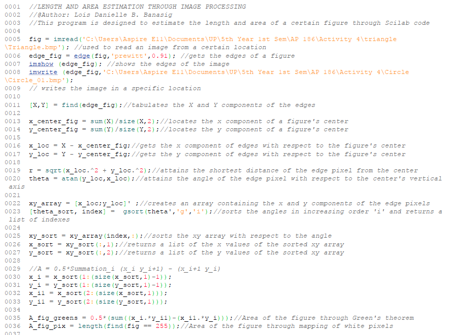
The Scilab code, as seen in the Fig. 2 below, was used to obtain the corresponding areas with varying edge detection methods, namely, Sobel, Prewitt, Canny, Log, and FFT Derivation methods.

Figure 2. The Scilab code for obtaining the approximate area of a circle, square, and triangle through pixel counting method and Green's theorem with 5 different edge detection methods (Sobel, Prewitt, Canny, Log, and FFT Derivation).

For the area approximation methods, the pixel counting method was found to be highly reliable for both the areas of the circle and the square with corresponding percent errors with the analytical area of only 0.0391 and 0.0000 respectively. The said method was found out to have a higher percent error of 0.3577 for the triangular image which can be accounted for the graphical errors observed in Fig. 3 upon zooming-in the triangle.

Figure 3. Zoomed-in image of the triangle showing the non-cohesive behavior of the hypotenuse pixels

It was observed that the created image using pain had non-cohesive diagonal pixels which decreased the accuracy of the area approximation methods. Upon applying the Green's theorem with edge detection for area approximation, varying accuracies were observed for different edge detection methods. This can be physically seen upon qualitatively analyzing the obtained edges for each corresponding method as seen in Figs. 4, 5, and 6.

Figure 4. Various synthetic images created using the edge detection of Scilab for a simple circular image. The (a) original image is initially shown and different methods namely the (b) Canny, (c) FFTDeriv, (d) Log, (e) Prewitt, and (f) Sobel edge detection method.

Figure 5. Various synthetic images created using the edge detection of Scilab for a simple square image. The (a) original image is initially shown and different methods namely the (b) Canny, (c) FFTDeriv, (d) Log, (e) Prewitt, and (f) Sobel edge detection method.

Figure 6. Various synthetic images created using the edge detection of Scilab for a simple triangular image. The (a) original image is initially shown and different methods namely the (b) Canny, (c) FFTDeriv, (d) Log, (e) Prewitt, and (f) Sobel edge detection method.

Out of all the detection methods, the most accurate method was the Log method (percent deviations ranging from approximately 0.1% to 0.2%)  which somehow sandwiches the edge with two lines: one for the inner line, and one for the outer line. The accuracy can be noticed upon zooming in the images. Due to the low image resolution, pixels tend to be non-cohesive and do not follow the expected (theoretical figure), which in return, results to an image with higher degree of error. Sandwiching the edges with inner and outer lines tend to decrease the errors brought by the pixel's non-cohesiveness for low-resolution images by means of error cancellation. The inner line gives a lower area and the outer line gives a greater area, resulting to a final averaged area with lower errors. The Prewitt and FFTDeriv methods were found to also be highly accurate with equal percent deviations ranging from 0.15% to 0.5%. The Canny method was also accurate but with higher percent errors ranging from 0.2% to 0.85% , while the Sobel method was found to have accuracy issues with errors ranging from 3% to 94%. The tabulated area values with their corresponding percent errors can be seen in Table 1 below.

Table 1. Approximated Area values with their corresponding percent deviations from the analytic value for different area approximation and edge detection methods.

For the part 2 of the activity, the approximation methods were extended in obtaining the area of a local building in UP Diliman, the CSRC, and the area of one of the largest cities in country, Quezon City. The use of Google Maps and Windows Snipping Tool was utilized, together with the Scilab code and Paint for distance scaling and area approximation. A snip of the local building/city was initially obtained from Google Maps and the distance and area measuring tool of the said application was used to obtain the approximate area of the said building (CSRC) or city (Quezon City). Paint was then used for distance scaling as done in Activity 2 of this blog and for monochrome image conversion. The process can be seen in Figs. 7, 8, and 9, wherein the approximate area of the CSRC building was obtained with the methods introduced.

Figure 7. A snip of the CSRC building obtained from Google Maps.

Figure 8. The obtained area and perimeter of the CSRC building using Google Maps' distance calculation function.

Initially, the theoretical value was obtained through the area and length approximation of Google Maps wherein the edges of the building was traced and scaled by the said application. The theoretical value was observed to be 1137.55 sq. meters as seen in Fig. 8.

Figure 9. Various synthetic images created using the observed 3 most efficient edge detection methods of Scilab for the CSRC building; namely, the FFT Derivation method (top), the Log method (middle), and the Prewitt method (bottom). A certain threshold values (right panes) were introduced to get more accurate representations as compared to the representations without the introduction of the said threshold (left panes).

The multiple area values were then obtained through the observed three most efficient edge detection methods namely, the FFT Derivation, Lod, and Prewitt methods, coupled with the algorithm of Green's Theorem in Equation 2. The pixel counting method was also used for its high area approximation efficiency, represented by the small deviation from the theoretical value. The area calculated by the pixel counting method was found to be equal to 1143.4 sq. meters which garnered a percent deviation of 0.5124% with respect to the theoretical value. Edge detection methods were found to be more accurate having lower deviations of 0.4598%, 0.4734%, and 0.4598% for the FFTDeriv, Log, and Prewitt methods respectively. Threshold values of 0.75, 0.552, and 0.91 were then applied to the same methods in similar order which produced more accurate area approximation values of 1142.7, 1142.3, and 1142.7 sq. meters having deviations equal to 0.4565%, 0.4182%, and 0.4554%, respectively. The Log method was again observed to be the most efficient area approximation method upon the application of Green's theorem. The deviations can be accounted by the errors in tracing the theoretical area of the building and the deviations resulted by the pixel scaling method used. 

Similar processes were also done in determining the approximate area of Quezon City and compared with the known theoretical value of 165.3 sq. km. as seen in Figs. 10, 11, and 12. The high irregularity of the city figure resulted to a much more complex process of pixel cleaning and scaling.

Figure 10. A snip of the whole Quezon City through Google Maps

The image was cleaned and monochromatic bitmap image was obtained through the use of Microsoft Paint as seen in Fig. 11. The approximate areas were then calculated by incorporating the Green's theorem with the selected edge detection methods as seen in Fig. 12. The pixel counting method was also found to be highly accurate with only about 6.57% deviation (area = 176.16 sq.km.) from the expected value. The application of Green's theorem with Scilab Image detection was also found to be accurate with about 6.72% (area = 176.42 sq.km.), 6.84% (area = 176.60 sq.km.), and 6.73% (area = 176.42 sq.km.) deviations for the FFTDeriv, Log, and Prewitt methods, respectively. Upon varying the threshold magnitudes, the accuracy was not that improved except for the FFT Derivation method. But as we examined the resulted synthetic image for the edges, it was found out that the accuracy was just an artifact due to the deviation from the expected image. This can be observed in Table 2 and Fig. 12. Here we suggest that the obtained image from Google Maps might have accuracy issues with the known area of Quezon City. Similarly, the scaling factor given by Google Maps might also not be that accurate when applied to larger areas.

Figure 11. Pixel cleaning and scaling for the monochromatic bitmap image of the ehole Quezon City area

Figure 12. Varied synthetic images formed through the three most efficient edge detection methods namely, the FFT Derivation (top), Log (middle), and Prewitt (bottom) methods. Threshold values (right panes) for image detection was applied to obtain more accurate area approximations as compared to the non-threshold approximations (left panes).

Table 2. The obtained approximate area values for the areas of the CSRC building and Quezon City with corresponding percent deviations.

For the final part of the activity, ImageJ was used to determine the approximate area of a known flat object such as a school ID. Here, a scanned personal UP Diliman ID card as seen in Fig. 13 was analyzed in ImageJ for area approximation. The scanned object was then edited and aligned through Windows 10 Photoviewer and Editor for higher contrast that will be essential for edge detection (seen in Fig. 14). The said object was then varied in image sizes and their corresponding areas were then obtained and checked with the theoretical value of 8.84 sq.cm (note that the area is not of the whole ID card but of the red box for ease of use and efficiency).

Figure 13. Scanned personal UP Diliman Identification Card

Figure 14. Edited UP Diliman ID card for alignment, scaling, and better contrast for edge detection. The image was also varied in size to obtain the dependence of the approximated area with the image size.

The results show that ImageJ can be a reliable tool for area and length approximation with errors varying from about 0.1% to 2%. It was also observed that the deviations are proportional to the image size as seen in Table 3. But I believe that this trend is just an artifact due to resolution and accuracy of the box tool used in ImageJ.

Table 3. UP Diliman ID card approximate areas obtained through ImageJ with varying image size percentages and corresponding percent deviations. 

I would like to thank the Musni Family for my long weekend Subic trip which helped me clear off my mind and allow me to be more productive the succeeding days. I would also like to thank my Adviser Dr. Rene Batac for understanding and being patient with my sickness, coupled with the moral support and academic guidance he gives.

Lastly, I would like to rate myself a 12/10 for the very rigorous parts done in not only one segment but in all segments of this activity. The complexity of each step allowed me to appreciate more hardwork and time-management in dealing with academic, family, and extra-curricular work. God bless and see you in my next blog post!